2.7. Example of a digital video filter

The following section introduces an example of a low-pass digital FIR filter for video applications, showing how power savings can be made by replacing multiplications with shift and add operations. This is possible by using a special format for the filter coefficients as powers of 2 or differences of powers of two. For digital realizations adders from section 2.5 have been used.

The same filter will be realized in Chapter 4 as an analog filter where comparisons between analog and digital realizations will be given. The filter has a pass-band up to 5.5MHz, a transition band from 5.5MHz up to 15MHz and a stop-band rejection better than -40dB. The specifications of the video filter are summarized in table 2.2. For a luminance video filter it is important to have a very low pass-band ripple. That is why the possible solutions are Butterworth and inverse-Chebyshev filters with a maximally flat amplitude in the pass-band. It is known that inverse-Chebyshev filters provide a smaller group-delay when compared to Butterworth counterparts. That is why, an inverse-Chebyshev filter has been chosen.

The synthesis procedure of the filter is given in Appendix 2 and the outcome of the synthesis is the filter from fig.2.13. The group delay of the filter varies from 46ns and 59ns, thus within specifications.

Pass-band edge	5.5MHz
Stop-band edge	14.8MHz
Stop-band rejection	³ 30dB
Group-delay	46ns£ t gr£ 65ns
Technology	0.5mm CMOS

Table 2.2: Video filter specifications

Fig.2.13: The LP prototype after scaling

The chosen sampling frequency of the filter is f_sampling=40MHz. As long as the coefficients are fixed, multiplications can be transformed in shift and add operations. The computed coefficients are given in table 2.3. Here T stands for sign inversion and L represents the exponent. The first column shows the coefficients in real format and in the second column, the coefficients are given in CSD (Carry sign digit) format.

Real notation	CSD notation
0.0000000000000L+00	0.0000000000000000
2.3437500000000L+00	0.000010T000000000
-3.9062500000000L-02	0.0000T0T000000000
-6.2500000000000L-02	0.000T000000000000
2.8906250000000L-01	0.0100101000000000
5.8203125000000L-01	0.1001010100000000
2.8906250000000L-01	0.0100101000000000
-6.2500000000000L-02	0.000T000000000000
-3.9062500000000L-02	0.0000T0T000000000
2.3437500000000L+00	0.000010T000000000
0.0000000000000L+00	0.0000000000000000

Table 2.3: Coefficients in real format and CSD format

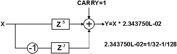
In this format (CSD), the coefficients are realized from powers of two or differences of powers of two. Multiplication with a power of two means shifting. Consider the second coefficient of the filter 2.343750L-02 which can be written as 1/2⁵-1/2⁷. The multiplication with this value is illustrated in fig.2.14.

Fig.2.14: Multiplication by hardwiring

Fig.2.15: Example of a FIR digital video filter

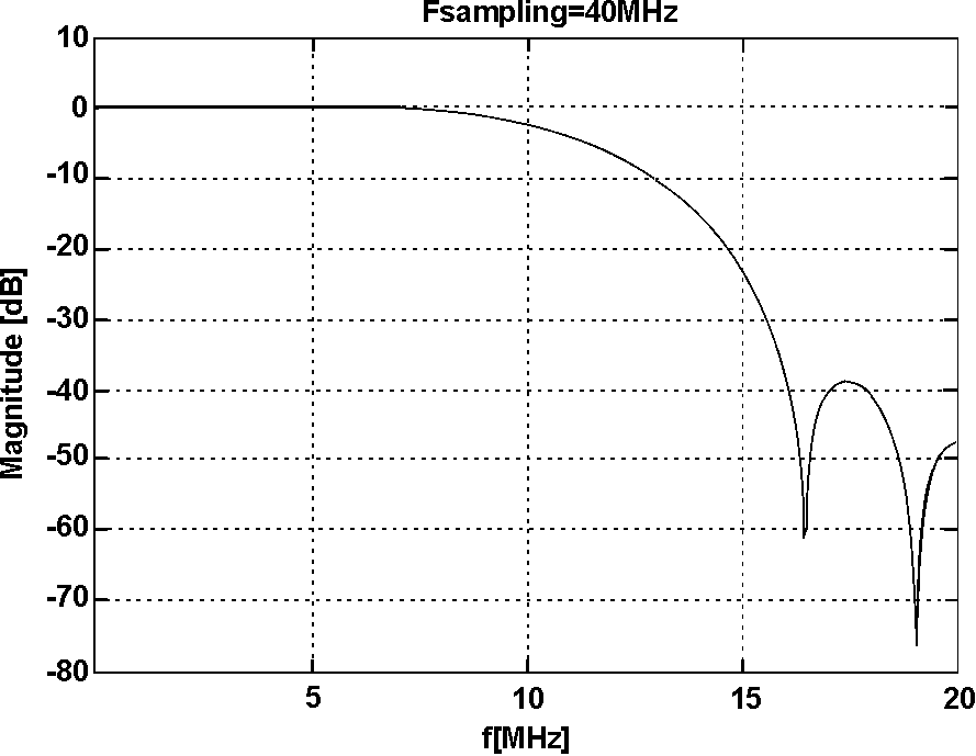
The input is shifted 5 times and added to the inverted value of the input shifted 7 times. The adder has one bit in plus compared to the word-length and the input CARRY set to one such that overflow will not occur. Fig.2.15 shows the transfer function of the video filter realized with coefficients from table 2.3. It is important to mention that CSD format is an approximation of the filter coefficients. That is why a computer routine is necessary to find the best approximation to fit the filter within the specifications. This method can be used whenever coefficients are fixed, like in dedicated applications.

According to table 2.3, the filter can be implemented with 11 adders for multiplications and 9 adders for final summation. The power consumption of the filter can be found by using the results of section 2.5. In the Table 2.4 the energy consumption of the full adder FA from fig.2.8 are given. The technology is a 0.5m m CMOS digital technology. The power consumption of the FIR video filter taking into account only the computational power is 2mW which gives about 660m W per pole (0.16pJ/pole). To be mentioned that FIR filters are all zero filters but for the sake of comparisons with analog approaches we have considered the power per analog pole.

In conclusion, this example shows that for applications with fixed coefficients a multiplier is not always necessary and power savings can be achieved by using only shift and add operations.

Eab	Eac	Ebc	PFIR/pole
56fJ	75fJ	84fJ	660m W

Table 2.4: Energy per transition of a full adder in 0.5mm CMOS